In 2019, AMD moved off their long-serving GCN architecture in favor of RDNA. We’ll cover the first generation of RDNA some other time. RDNA 2 takes that foundation and scales it up while adding raytracing support and a few other enhancements. We already covered compute aspects of the RDNA 2 architecture in a couple of other articles, in order to make comparisons with other architectures. So, I figured we could do something fun and look at some games from RDNA 2’s perspective.

Architecture

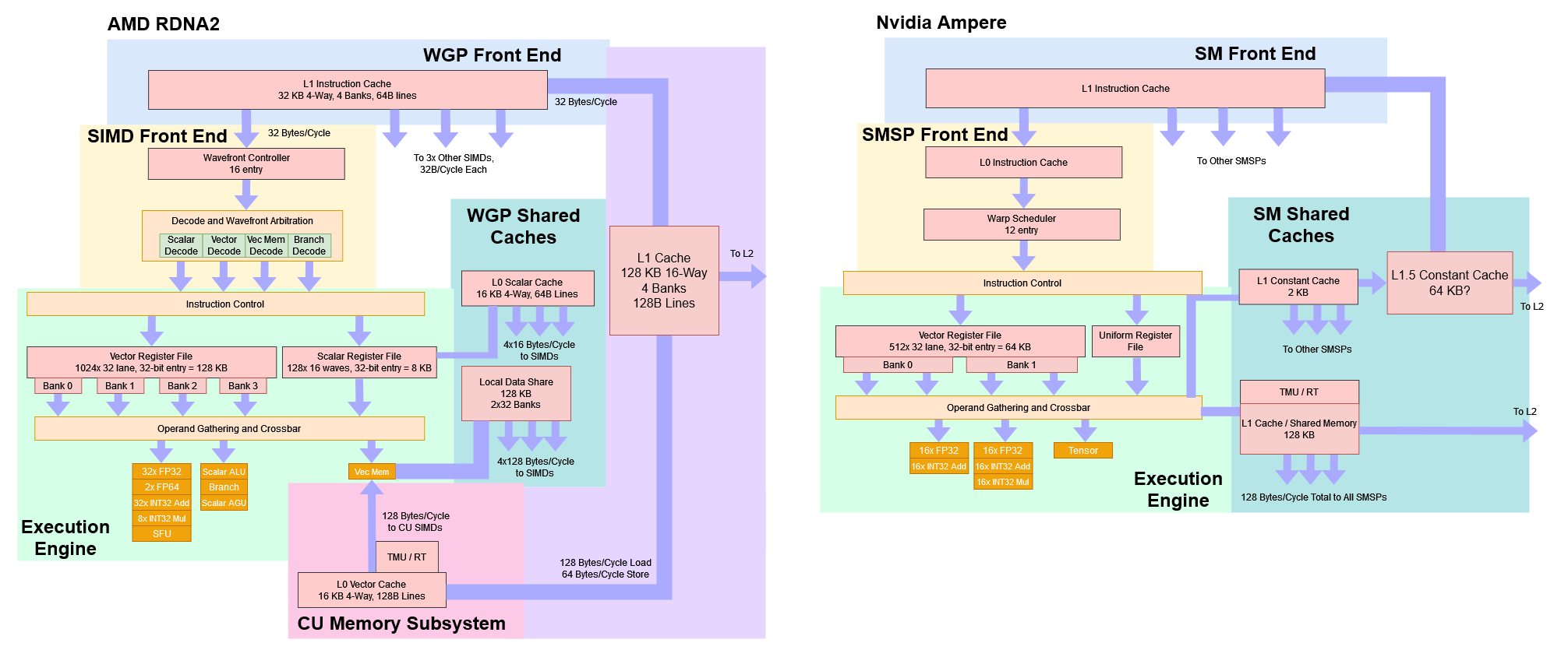
As its name implies, RDNA 2 builds on top of the RDNA 1 architecture. AMD made a number of changes to improve efficiency and keep hardware capabilities up to date, but the basic WGP architecture remains in place. Each WGP, or workgroup processor, features four SIMDs. Each SIMD has a 32-wide execution unit for the most common operations. RDNA 2 gets a few extra instructions for dot product operations to help accelerate machine learning. For example, V_DOT2_F32_F16 multiplies pairs of FP16 values, adds them, and adds a FP32 accumulator. It doesn’t go as far as tensor cores on Nvidia, where instructions like HMMA directly deal with 8×8 matrices. But those instructions let RDNA 2 do matrix multiplication with fewer instructions than if it had to use plain fused multiply-add instructions.

Each SIMD has 32-wide execution units for the most common operations, a 128 KB vector register file, and can track up to 16 wavefronts. AMD therefore reduced the number of wavefronts RDNA 2 could track, from 20 in RDNA 1. GPUs don’t do out of order execution the way high performance CPUs do. Instead, they keep a lot of threads in flight, and switch between threads to keep the execution units occupied to hide latency. On RDNA 2, a SIMD basically has 16-way SMT, versus 20-way on RDNA 1.

That might sound like a regression, but tracking more wavefronts (analogous to CPU threads) is probably expensive. Thread or wavefront selection logic has to solve a very similar problem to CPU schedulers. Every cycle, every entry must be checked to see if it’s ready for execution. AMD probably wanted to reduce the number of checks per cycle from 20 to 16, in order to hit higher clock speeds at lower power. RDNA 2 clocks much higher than its predecessor on the same process node, so AMD did a good job there.

RDNA 2 also compares well to Ampere. Even though both architectures use basic building blocks (SMs or WGPs) that can do 128 FP32 operations per cycle, a RDNA 2 WGP can keep 64 wavefronts in flight. An Ampere SM can only keep 48 warps in flight. RDNA 2 also has more vector register file capacity, meaning the compiler can keep more data in registers without reducing occupancy.

Architecture	Waves Per SIMD/SMSP	Vector Registers Per SIMD/SMSP	Registers Available for Max Occupancy
RDNA 2	16 (wave32)	128 KB	64
RDNA 1	20 (wave32)	128 KB	51
GCN	10 (wave64)	64 KB	25
Ampere	12 (32-wide warp)	64 KB	42

That gives a RDNA 2 WGP a better chance of being able to hide latency, by keeping more work in flight. Combine that with better caching, and each RDNA 2 WGP should be able to punch harder than an Ampere SM.

A WGP’s four SIMDs are organized into groups of two, which AMD calls compute units (CUs). A CU has its own memory pipeline and 16 KB L0 vector cache. At the CU level, AMD augmented the memory pipeline to add hardware raytracing acceleration. Specifically, the texture unit can now perform ray intersection tests, at a rate of four box tests per cycle or one triangle test per cycle. Box tests take place at upper levels of the BVH, while triangle tests happen at the last level. A BVH, or bounded vertex hierarchy, speeds up raytracing with a divide-and-conquer methodology. Because checking every triangle in a scene would be extremely expensive, box tests narrow down what area a ray goes through, and ideally the GPU only checks a narrow set of triangles in the end.

Raytracing acceleration is accessed via a couple of new texture instructions. Obviously these instructions don’t actually do traditional texture work, but the texture unit is a convenient place to tack on this extra functionality. The new instructions themselves don’t do anything beyond an intersection test. Regular compute shader code deals with traversing the BVH. It also has to calculate the inverse ray direction and provide that to the texture unit, even though the texture unit has enough info to calculate that by itself. AMD probably wanted to minimize the hardware cost of supporting raytracing, and figured they had enough regular shader power to get by with such a solution.

Caching

Beyond going for feature parity with Nvidia, RDNA 2 scales up to reach performance parity. The highest end RDNA 1 GPU, the RX 5700 XT, only has 20 WGPs. It’s also built on a small 251 mm² die, and competes with Nvidia’s midrange cards rather than challenging their highest end ones. RDNA 2’s RX 6900 XT doubles WGP count and increases clock speed, showing AMD’s ambition to take a shot at Nvidia’s best. But just like increasing core counts on a CPU, scaling up a GPU creates higher bandwidth demands. Nvidia opted for a power hungry 384-bit GDDR6X setup to feed Ampere. AMD however chose to stick with a 256-bit GDDR6 configuration. To avoid memory bandwidth bottlenecks, RDNA 2 gets an extra level of cache. AMD dubs this “Infinity Cache”, and internally refers to it as MALL (memory attached last level).

The MALL designation makes sense because all VRAM accesses go through it. RDNA 2’s L2 is also a single cache shared by the entire GPU, but can be bypassed if virtual memory pages are set to uncached. Synchronization barriers can also flush L2 to ensure coherency. Those accesses could be caught by the Infinity Cache on RDNA 2, while previous AMD GPUs would service them from VRAM.

Because the L2 should be large enough to catch the bulk of memory accesses, Infinity Cache performance isn’t as important and AMD runs the Infinity Cache on a separate clock domain. That means it can be clocked lower to save power.

Latency

Using a latency test, we can see AMD’s complex four-level cache system in action. We can also see Nvidia’s simpler two-level cache hierarchy. Ampere’s SMs have more L1 caching capacity, letting a SM service requests from its first level cache when RDNA WGPs would have to do so from the slower per-SA L1. At larger test sizes, RDNA 2 has a clear latency advantage especially when test sizes spill out of Nvidia’s L2.

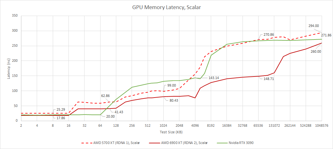
Compared to RDNA 1, the first three cache levels see minor performance gains, mostly from increased clock speeds. Then Infinity Cache makes a huge impact at larger test sizes. Latency is impressively low for such a large cache. For comparison, the RTX 3090’s L2 has 140 ns of latency, but only 6 MB of capacity.

Infinity cache latency also deserves a closer look. AMD’s Adrenaline Edition software is quite advanced and lets users set almost arbitrary maximum clock speeds. We can use that to see how the cache behaves as GPU core clocks vary.

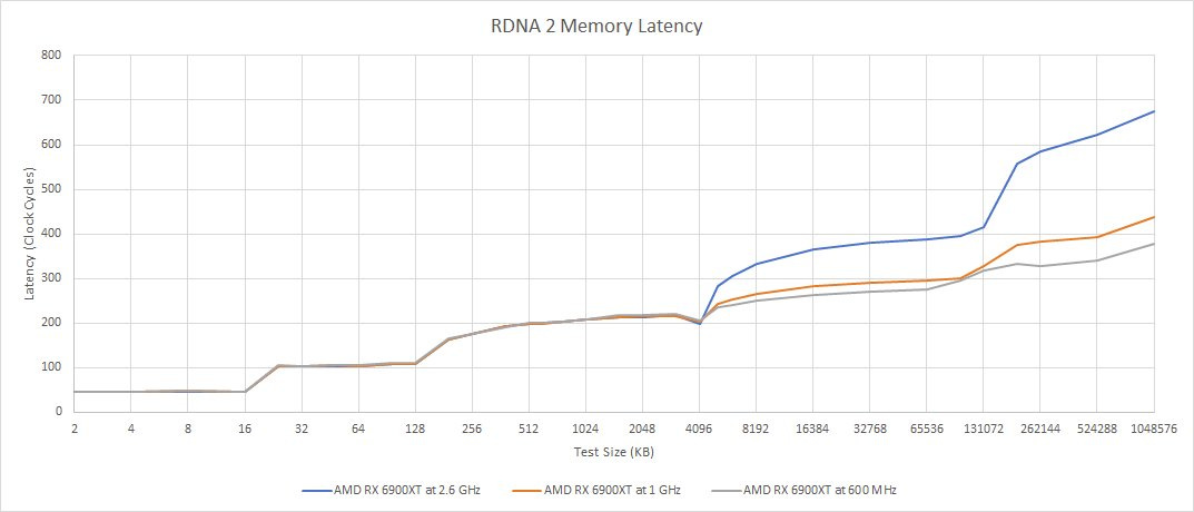
At lower clocks, RDNA 2’s WGPs take fewer cycles to get data from Infinity Cache. That could mean improved shader utilization at lower clocks.

From the vector side, we see the same story. RDNA 2 is a lot like a faster RDNA 1, with an extra gigantic cache bolted on. Vector accesses are higher latency than scalar ones. Nvidia doesn’t have a separate scalar memory hierarchy. Their architectures do have constant caches, but those are read only and serve a more limited purpose than AMD’s scalar datapath.

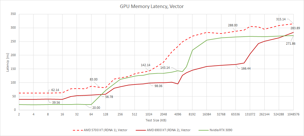
Nvidia benefits from lower latency for small test sizes, while RDNA 2 maintains an advantage at larger test sizes. AMD’s L2 and Infinity Cache latency look very good, considering RDNA 2 has to check more cache levels than Nvidia. The situation flips back around once we get to VRAM.

Bandwidth

Bandwidth is important too, because GPUs are designed to process lots of operations in parallel. Let’s start by looking at bandwidth from a single workgroup. Running a single workgroup limits us to a single WGP on AMD, or a SM on Nvidia architectures. That’s the closest we can get to single core bandwidth on a CPU. Like single core bandwidth on a CPU, such a test isn’t particularly representative of any real world workload. But it does give us a look into the memory hierarchy from a single compute unit’s perspective.

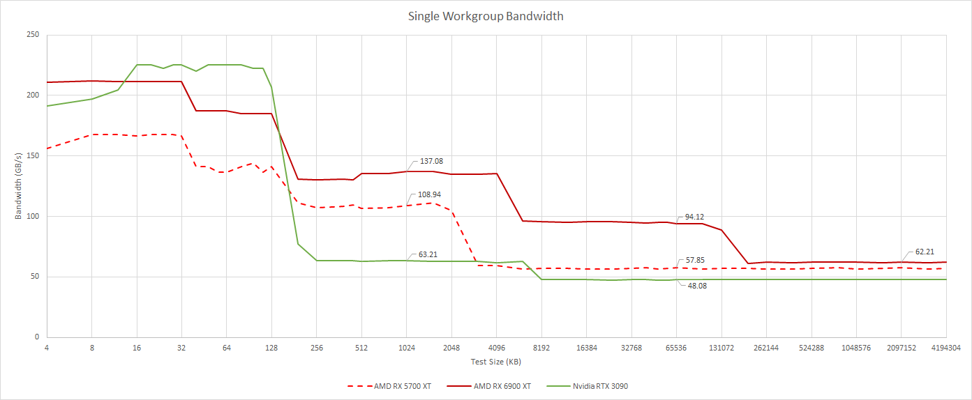
From a single WGP, RDNA 2 achieves very high cache bandwidth thanks to high clocks. This advantage is especially prominent at large test sizes, where the 128 MB Infinity Cache comes into play. AMD’s cache architecture is a lot better than Nvidia’s here. At low occupancy, even Infinity Cache can provide more bandwidth than Ampere’s L2.

As we use more workgroups and load more WGPs or SMs, bandwidth demands obviously go up. That puts heavier demands on shared caches. AMD does a very good job here. L2 bandwidth starts excellent and scales very well as we load up more WGPs. We have to load up a lot more SMs on Nvidia’s RTX 3090 before we start getting good bandwidth.

Infinity Cache bandwidth scales very well too, and actually closely matches RDNA 1’s L2 bandwidth. It can’t match L2 bandwidth on Nvidia’s 3090, but it doesn’t need to because the 4 MB L2 in front of it should catch a lot of accesses. So far, AMD looks pretty good in terms of cache bandwidth. VRAM however, is another story.

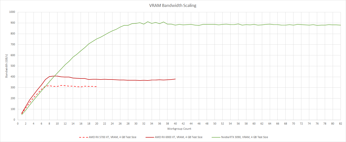
Nvidia has a massive VRAM bandwidth advantage. With large workloads that don’t fit in cache, Ampere is far less likely to run out of VRAM bandwidth. However, both RDNA generations are better at making use of the VRAM bandwidth they do have. They don’t need as much work in flight to make good use of their available bandwidth.

CU and WGP Mode

The WGPs in AMD’s RDNA architecture can operate in both WGP mode, and CU mode. In WGP mode, the 128 KB LDS works as a single unified block of memory. All four SIMDs within the WGP can access the entire 128 KB. In CU mode, the LDS is split into two 64 KB halves, each associated with a pair of SIMDs.

LDS latency stays the same in both modes at around 19.5 ns, even though CU mode should simplify request routing from the LDS. The same applies to RDNA 1, which has about 26.6 ns of LDS latency.

The LDS organization difference lets us hit a single CU (half of a WGP) by testing with a single workgroup. Because each CU has its own memory pipeline and L0 cache, we see a drop in L0 bandwidth when we’re only using one CU in the WGP. There’s no drop in bandwidth once we get to L2 on beyond.

That’s a large improvement over RDNA 1, which sees a significant drop in bandwidth further down the cache hierarchy. Bandwidth is often a function of how well queues can hide latency, so perhaps RDNA 2 is more flexible in how it can allocate queue entries. Maybe some queues between L1 and L2 were allocated per-CU in RDNA 1, but are allocated per-WGP in RDNA 2. To GPU workloads, that means RDNA 2 performs better if waves running in one half of a WGP finish early.

From the Gaming Perspective

RDNA 2 is a gaming first architecture, so let’s look at what the RX 6900 XT has to deal with in those workloads. Looking at gaming will also help us understand what gaming workloads look like.

Cyberpunk 2077, RT On

CD Projekt Red’s Cyberpunk 2077 is a showcase of modern GPU technology. It uses DirectX 12 with plenty of raytracing to provide a wealth of graphical effects. Unfortunately, these effects can be very heavy. Raytracing takes an especially large toll on performance. Keep in mind numbers for this game were obtained with the GPU’s maximum clock set to 1800 MHz for consistency. The 3950X had boost disabled. So, numbers here shouldn’t be taken as stock performance figures, and shouldn’t be compared with other systems. We’re only looking at what kind of work the card is doing. In this game, we’ll be looking down Jig Jig street.

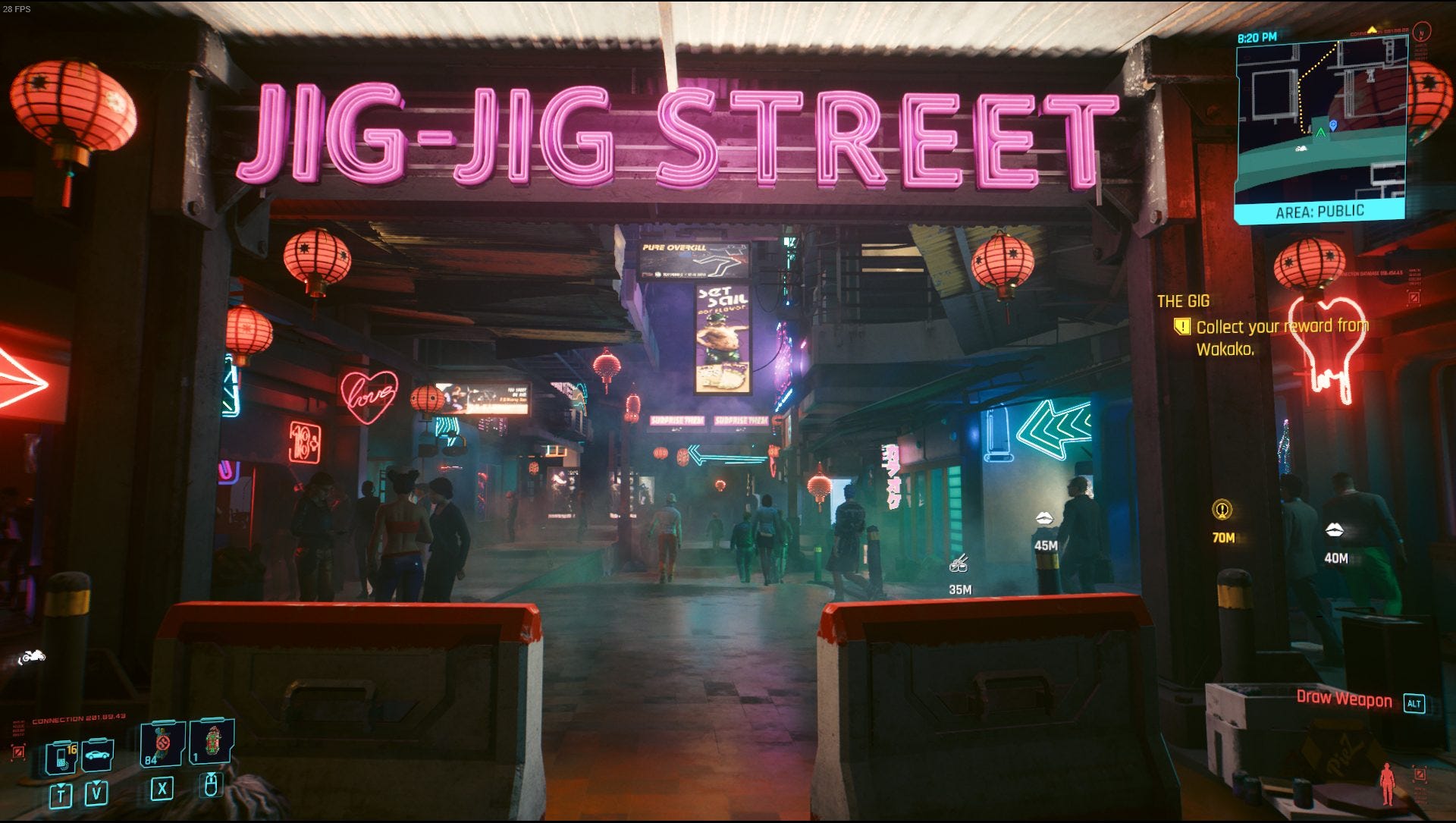
RT-related work takes up around 21 ms of frame time. Over 9 ms of that is spent building the BVH, so optimizing BVH build time is almost as important as optimizing BVH traversal. To render raytraced effects, the 6900 XT had to do 580 million box intersection tests, and 109.5 million triangle intersection tests. At the achieved 25.9 FPS, that’s 15 billion box tests and 2.8 billion triangle tests per second.

Besides raytracing, Cyberpunk makes heavy use of compute. Traditional rasterization takes a back seat, perhaps showing a trend with cutting edge games. Because most of the time is spent doing raytracing, let’s take a closer look at that starting with the longest running DispatchRays call. Specifically, let’s check out the one that takes 7.2 ms, all by itself:

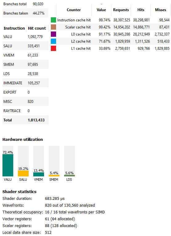
Internally, RDNA 2 treats raytracing kernels as compute shaders. This particular call launched 32,400 compute wavefronts. The 6900 XT’s 40 WGPs can keep a total of 2560 wavefronts in flight, so this is more than enough work to fill the entire GPU. However, RDNA 2 can’t keep 2560 of this kernel’s wavefronts in flight, because it doesn’t have enough vector register file capacity. Unlike CPUs, GPUs flexibly allocate vector register file capacity. Giving each thread (wavefront) more registers can help prevent register spilling, but also reduces the number of threads it can keep in flight.

For this kernel, the compiler chose to use 96 vector registers, meaning RDNA 2 only has enough vector register file capacity to track 10 wavefronts per SIMD, or 1600 across the entire GPU. On one hand, that means each SIMD has less capability to keep execution units busy by switching between wavefronts when one stalls. On the other, using more registers could let the compiler expose more instruction level parallelism. From the profile, RDNA 2 spends a lot of time with occupancy limited by vector register capacity, so reducing maximum occupancy from RDNA 1 looks justified.

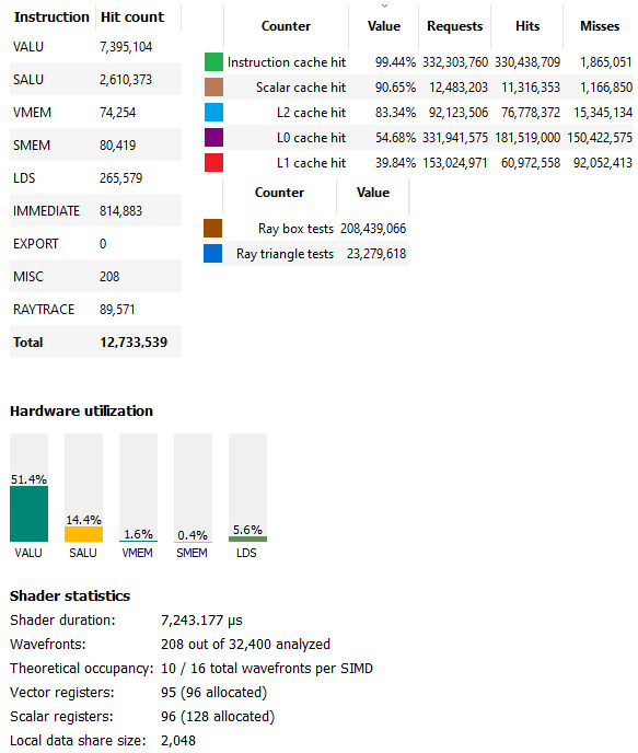
In this case, the driver probably made the right tradeoff, or at least didn’t make a bad one. 51% vector ALU usage is in a good place to be. The shaders are not under-utilized. At the same time, utilization doesn’t push over 70-80%, which would suggest a compute bound scenario. We also see light LDS usage. AMD uses the LDS to store the BVH traversal stack, keeping writes and latency-sensitive reads off the less optimized global memory path. Other raytracing calls show similar hardware utilization patterns.

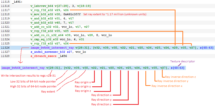
Here’s a basic block from the shader that hits the RT units. The shader has to use three extra instructions to calculate the inverse of the ray direction, and provide that alongside the ray direction. Three extra instructions isn’t much, but these reciprocal instructions are rather expensive and only execute at quarter rate compared to simpler FP32 operations. On top of that, the compiler has to use three extra registers to hold the inverse ray direction. I’m not sure how much of an impact this makes, but there’s room for improvement.

Unfortunately AMD does not expose Infinity Cache counters through their profiling tools. However, we can still look at how the first three cache levels do. To start, L0 cache hitrate is poor at just under 55%. CPUs usually see well over 80% first-level cache hitrate even in sub-par implementations like Bulldozer. The 128 KB mid-level cache helps catch some of those misses, bringing cumulative L0+L1 hitrate to just under 73%. My impression here is that the L0 and L1 caches are too small. The 4 MB L2 is a hero here, bringing cumulative hitrate to 95.4% before going out to the higher latency Infinity Cache.

RDNA 2’s 16 KB scalar cache achieves relatively good hitrate at just over 90%, and more importantly offloads some requests from the vector path. From the instruction side, the L1i gets over 99% hitrate. GPU programs seem to have smaller instruction footprints than CPU ones, and the 32 KB L1i appears adequate.

BVH Building

RGP annotates several sections as calls to BuildRaytracingAccelerationStructure, which builds the BVH. As noted before, these sections consume a significant portion of raytracing time, so let’s look at one of those too. The longest one is call number 4838, which strangely is a DispatchRays call and shows intersection test activity. I’m not sure what that means, so I’ll move on to the second longest one.

Call 4221 corresponds to CmdDispatchBuildBVH, and ran in the compute queue. It exhibits very poor occupancy because only 160 wavefronts were launched. That’s nowhere near enough work to fill the GPU, so this section is likely latency bound. A synchronization barrier prevents the GPU from using async work to keep the execution units busy. Fortunately, this section only lasts for 1.7 ms.

Unlike the ray traversal section covered above, AMD’s driver opted to use wave64 mode for this BVH building section. I doubt this is the best choice. wave32 mode should be preferable at low occupancy, because it’ll allow more thread level parallelism. But AMD probably had a good reason to use wave64, so I’ll stop being an armchair quarterback and move on to caching.

As before, instruction cache hitrates are very high. There’s not enough scalar memory accesses for the scalar cache to matter. On the vector side, the 16 KB L0 performs very poorly with less than 25% hitrate, and the 128 KB L1 may as well be absent. RDNA’s L2 ends up servicing most of the memory traffic, and in a more extreme way than with the ray traversal part. Because occupancy is so low, and L0/L1 cache hitrates are so poor, L2 latency is likely to be a limiting factor when building the BVH.

Compute

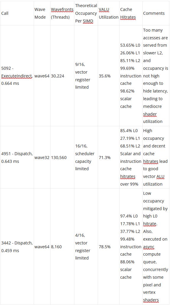
Besides raytracing, which is technically treated as a form of compute on RDNA, Cyberpunk 2077 makes heavy use of compute shaders. Non-raytracing compute in this game tends to consist of a lot of short duration calls, rather than a few very heavy ones. The longest duration compute call (number 4473) was compiled for wave32 mode, and runs for just under 0.7 of a millisecond. RDNA 2 eats this one for lunch. The shader doesn’t use a lot of vector registers or LDS space, and launches 130,560 wavefronts. As a result, occupancy is excellent.

Vector ALU utilization is very good as well. In fact, it’s almost too good. Any higher, and we would be calling this section compute limited. RDNA 2’s scalar datapath plays a critical role here in offloading calculations that apply across the wavefront. Cache hitrates contribute to good compute utilization too. About 94% of vector accesses were serviced by the L0 and L1 caches, with the bulk of those coming from L0. The L2 brings cumulative hitrate to over 98%. L1 instruction cache and scalar cache hitrates are so high that misses are basically noise. For this shader, good cache hitrates and high occupancy combine to let RDNA 2 shine.

The second longest compute shader (number 4884) ran for just under half a millisecond, and exhibits different characteristics. It uses wave64, and occupancy is limited by vector register file capacity to just four waves per SIMD. Despite that, RGP still reports very good VALU utilization. That’s likely because this kernel overwhelmingly consists of vector ALU instructions. There aren’t a lot of memory accesses, and a good chunk of the memory accesses that do happen go to the scalar path.

Moreover, this compute shader has very few branches, and RGP did not pick up any taken branches. Branches are quite expensive on GPUs, which don’t have branch prediction and must stall a thread until the branch condition is resolved. The lack of taken branches also implies divergence is not a big issue. Overall, this shader largely consists of straight-line FP32 spam. GPUs love that stuff. RDNA 2 is no exception, and achieves very good hardware utilization despite low occupancy.

Cyberpunk 2077, RT Off

Raytracing effects are cool, but Cyberpunk 2077 still looks really good with RT off. Traditional rasterization can still render impressive scenes if artists and developers are good at their job, and the people who worked on CP2077 definitely seem up to the task.

Without raytracing, traditional vertex and pixel shaders step in and play a much bigger role. However, the game still heavily uses compute shaders, and async compute shows up too. The three longest duration calls are all compute, summarized below:

Call	Wave Mode	Wavefronts (Threads)	Theoretical Occupancy Per SIMD	VALU Utilization	Cache Hitrates	Comments
5092 – ExecuteIndirect, 0.664 ms	wave64	30,224	9/16, vector register limited	35.6%	53.65% L0 26.06% L1 85.11% L2 99.69% instruction cache 98.62% scalar cache	Too many accesses are served from slower L2, and occupancy is not high enough to hide latency, leading to mediocre shader utilization
4951 – Dispatch, 0.643 ms	wave32	130,560	16/16, scheduler capacity limited	71.3%	85.4% L0 27.19% L1 68.51% L2 Scalar and instruction cache hitrates over 99%	High occupancy and decent cache hitrates lead to good vector ALU utilization
3442 – Dispatch, 0.459 ms	wave64	8,160	4/16, vector register limited	78.5%	97.4% L0 17.78% L1 37.77% L2 99.48% instruction cache 88.06% scalar cache	Low occupancy mitigated by high L0 hitrate. Also, executed on async compute queue, concurrently with some pixel and vertex shaders

RDNA 2 puts in a very good showing in these compute kernels, even if utilization is on the low side for the longest running kernel. Vector register file capacity continues to limit how much parallelism the architecture can take advantage of, but this problem isn’t unique to AMD. On the caching front, the 128 KB L1 often does badly. We saw that a 256 KB mid-level cache is already pretty mediocre for CPUs. GPU caching is even harder. Time and time again, RDNA 2’s L1 sees more misses than hits. I’m glad AMD chose to double L1 cache capacity in RDNA 3. On the bright side, scalar and instruction cache hitrates continue to be good.

Rasterization

Unlike raytracing, the traditional rasterization pipeline is very efficient. Instead of sending off rays everywhere and seeing what they hit, rasterization can use simple calculations to map 3D points into 2D screen space. Then, the GPU uses fixed function hardware to distribute work to pixel shaders, which determine what color those pixels should be. Like before, let’s look at a couple of the longest rasterization calls in CP2077.

Kernel	Wave Mode	Wavefronts (Threads)	Theoretical Occupancy per SIMD	VALU Utilization	Cache Hitrates
5112 – DrawInstanced 0.392 ms, nearly all pixel shader time	Vertex: wave32 Pixel: wave32	Vertex: 1 Pixel: 64,800	Vertex: 16/16 Pixel: 10/16, vector register limited	68.1%	80.85% L0 41.83% L1 43.55% L2 99.01% Instruction Cache 97.47% Scalar Cache
5102 – DrawInstanced 0.192 ms, nearly all pixel shader time	Vertex: wave32 Pixel: wave64	Vertex: 1 Pixel: 16,200	Vertex: 16/16 Pixel: 5/16, vector register limited	N/A, didn’t run for long enough for RGP to provide an estimate	91.5% L0 30.33% L1 22.48% L2 98.81% Instruction Cache 97.22% Scalar Cache

With rasterization work, the L1 cache puts in a more credible showing. Hitrates still aren’t great, but in some cases it’s catching enough L0 misses to ensure that the vast majority of requests don’t have to be satisfied from L2 or beyond. That can be a big advantage, because L1 latency and bandwidth characteristics are much better than the L2’s.

There’s also a cluster of vertex shader work close to the start of the frame. It’s hard to analyze because there are a ton of tiny calls, but peeking at a few shows that they often launch fewer than 100 wavefronts each. From our latency and bandwidth scaling tests, RDNA 2 is a very strong performer at low occupancy, and likely copes with those calls better than Nvidia’s Ampere would.

Titanic Honor and Glory, Megademo 401 (Rasterization, 4K)

Large studios with multi-million dollar budgets can produce complex games with many deep storylines and impressive visuals. But they don’t have a monopoly on fun, and independent creators on smaller budgets can create immersive and visually stunning stuff too. One such example is the work-in-progress Titanic Honor and Glory project, which focuses on recreating the Titanic in 3D. It uses Unreal Engine, and runs using DirectX 12.

Like many independent games, the developers have less time and resources to spend on optimization. But perhaps because it hasn’t been optimized, the demo has a stunning level of detail and is very heavy even on modern GPUs.

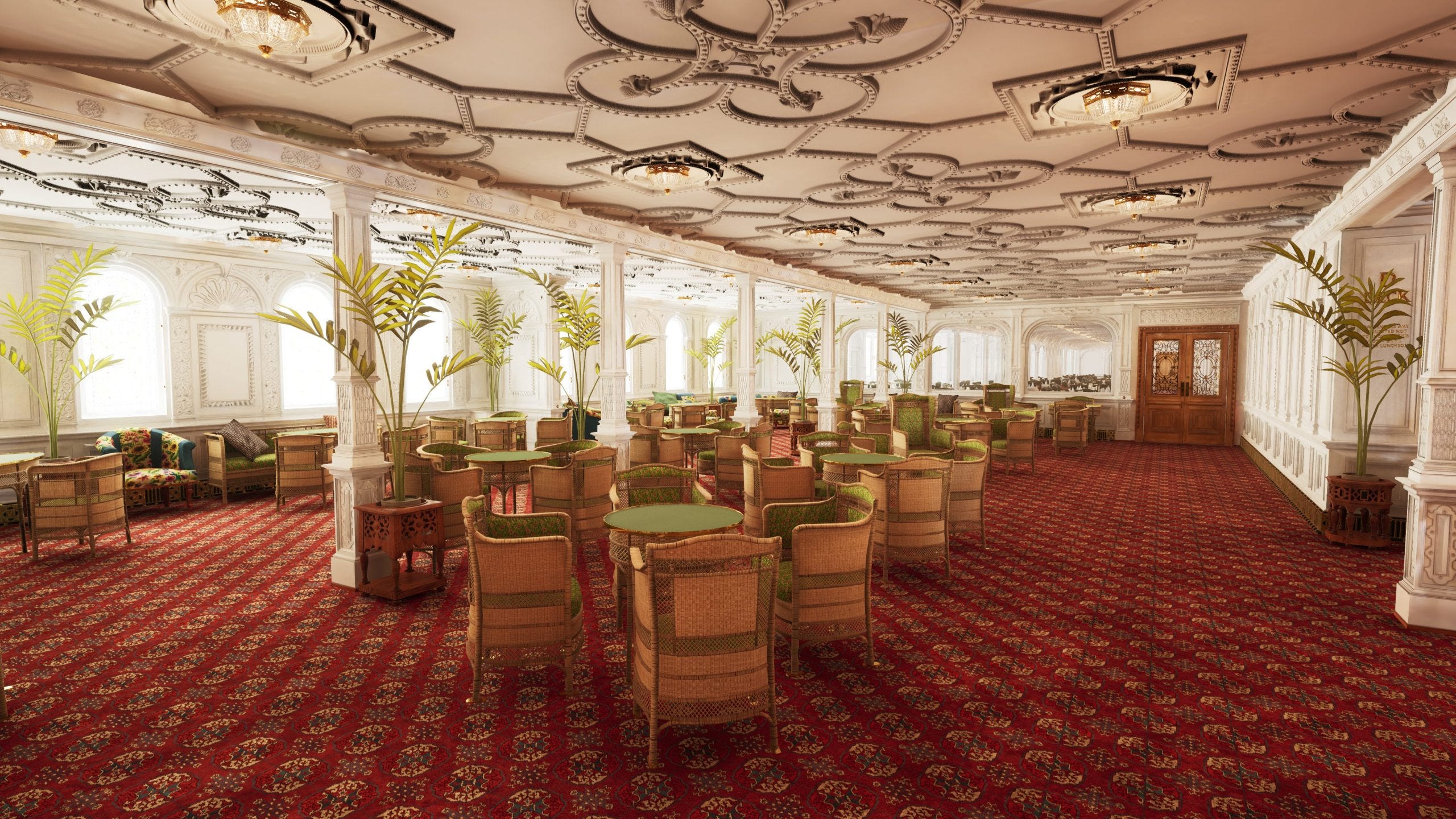
Here, we’re looking down the first class lounge with the game running at 4K, and GPU/CPU clocks set as before. Pixel shaders dominate this workload, but compute shaders do play a role too. Async compute usage is minimal, with almost all calls happening on the graphics queue.

The longest call is event 1325, a pixel shader running in wave64 mode. It launched 129,652 wavefronts, or enough waves to cover every pixel at 4K. Occupancy is low due to vector register file limitations. Vector ALU utilization is also poor, likely due to the combination of poor occupancy and mediocre cache hitrates.

Event 1330 is the second longest call, and is a compute shader that launches 16,320 wave32 wavefronts. Occupancy is again limited by the vector register file, but this time it’s better at 12 waves per SIMD. The shader achieves 27.7% vector ALU utilization, which is more acceptable but still on the low side. L0 hitrate is alright at 59.69%, while L1 hitrate is an embarrassingly low 13.11%. Fortunately, the L2 cache saves the day with 99.82% hitrate. Compute utilization should really be better because 12 waves per SIMD isn’t terrible occupancy. But a closer look reveals another problem. Work isn’t evenly distributed between threads, and some finish before others.

Apparently the next call needs data written by the compute shader, so a synchronization barrier prevents it from executing until all the threads in the compute shader have finished executing. Toward the end, that means many of the 6900 XT’s WGPs are idle or don’t have enough thread level parallelism left to effectively hide latency. That’s not great for any GPU, but RDNA 2’s high clock speeds and better handling at low occupancy should let it cope better than say, Nvidia’s Ampere.

With THG, we can see DirectX12 in action with rasterization. It doesn’t do raytracing like Cyberpunk 2077, but cache behavior is surprisingly similar across both workloads.

Gunner, HEAT, PC

Gunner, HEAT, PC (GHPC) is tank simulation indie game. It aims to accurately depict fire control systems and sensors on late Cold War tanks, while being more accessible than something like DCS. Unlike the THG demo, GHPC uses the Unity engine and runs off DirectX 11. AMD’s profiler unfortunately does not support DirectX 11. I used PIX to profile the game. But that has been quite annoying because PIX has a nasty habit of crashing both itself and the game it’s trying to profile.

GHPC overwhelmingly uses traditional pixel and vertex shaders. I’m running the game at 4K, so unsurprisingly there’s a lot of pixel shader work. Compute shaders are used. But unlike the DirectX 12 workloads above, they play a very minor role.

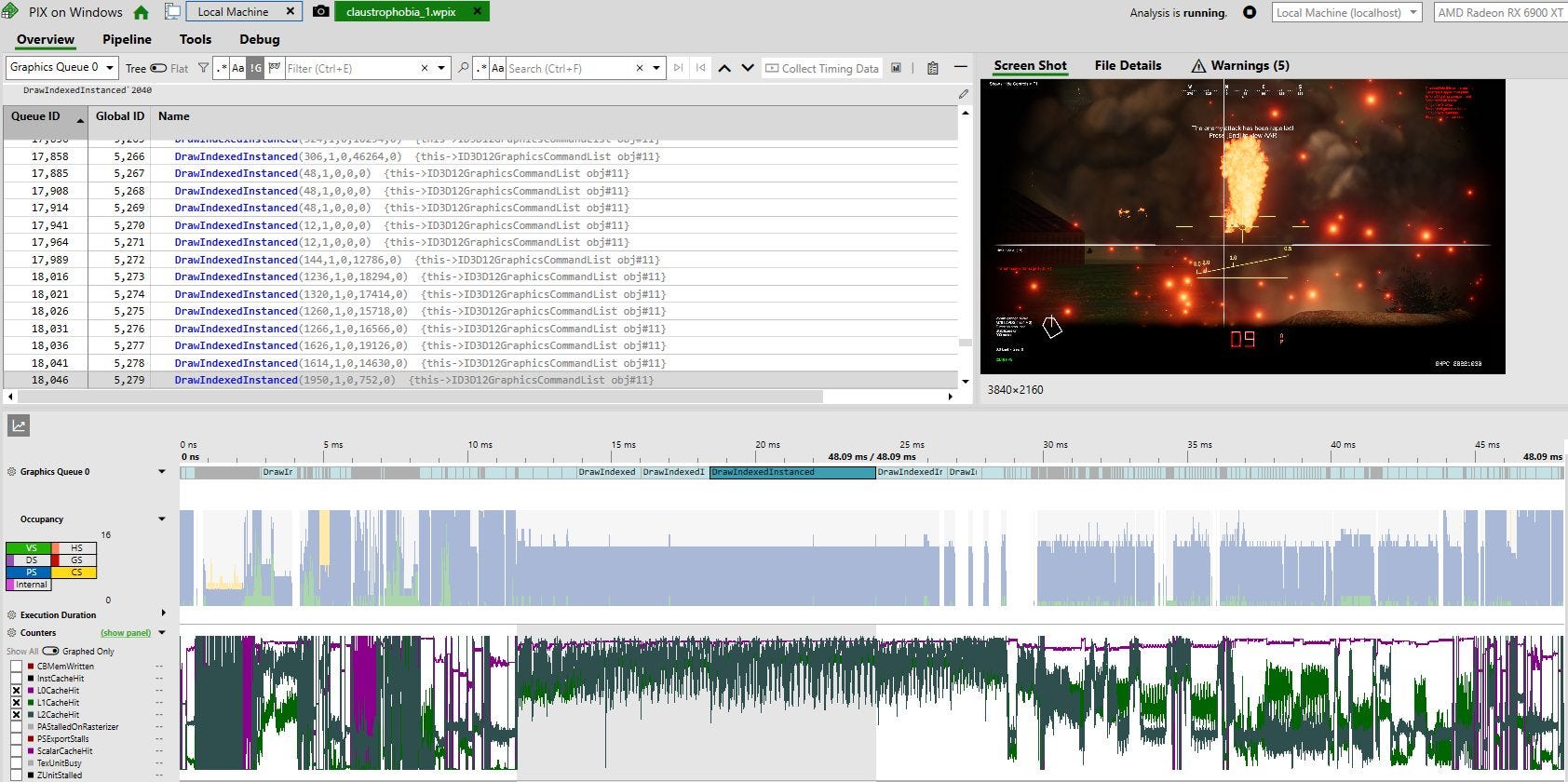
GHPC’s longest running pixels shaders are far more cache friendly than THG’s. We see over 90% L0 hitrate. L1 hitrate is finally excellent at 70-80%, and L2 hitrate oscillates between over 90% and around 60%. Scalar and instruction cache hitrates are basically 100%. Unfortunately PIX doesn’t show metrics on execution unit utilization, but I expect it to be quite good. That’s because game tends to make the card generate a lot of heat, even when running below stock clock speeds. Fortunately, PIX does expose far more counters than RGP does, so we can look into other aspects of the rasterization pipeline.

The long running pixel shader is compute bound, and seems to deal with drawing smoke effects. Calls early in the frame mainly deal with drawing objects, like houses and roads. Because those calls are short, and often overlap with each other, we see some rasterization bottlenecks show up. “PAStalledOnRasterizer” means that the primitive assembler is generating primitives faster than the rasterizer handle them. That could indicate a bottleneck at the rasterizer or anywhere after.

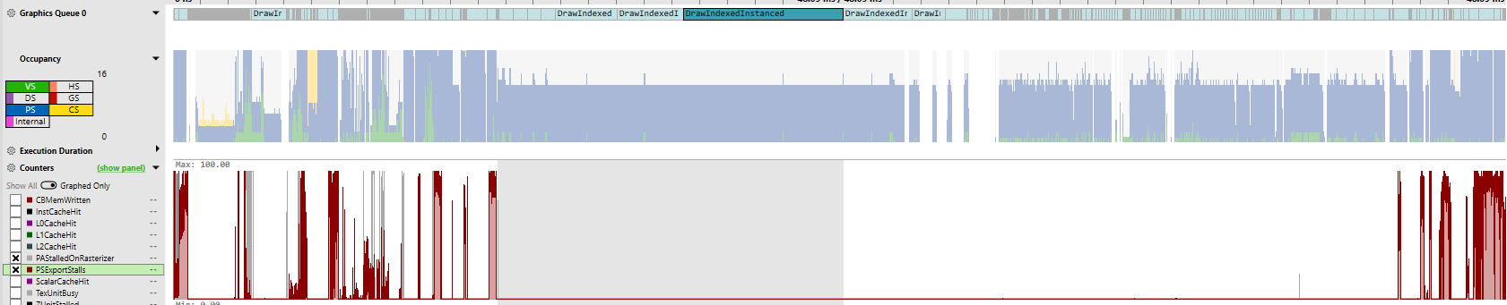
Another metric is “PSExportStalls”, which indicates when pixel shader programs have calculated color information, but the final stages in the rasterization pipeline aren’t ready to accept the data. One culprit is the Z unit, which does depth tests to make sure only non-occluded pixels are displayed. For example, if half of a tank is sitting behind a house, the Z-unit part would make sure the house’s pixels are displayed in the final frame. If a lot of pixels from many different objects have to go through this depth testing, perhaps it’s hard for the Z unit to keep up.

But zooming back out, the biggest performance culprits are definitely smoke and haze effects. Drawing those effects take up the most GPU time, and are very heavy on pixel shader operations. The texture units are active pretty much the entire time during those shaders, so there could be a texturing bottleneck too.

Caching Comments

For a long time, GPU caching trailed behind CPU caching. In the early 2000s, GPUs didn’t have a general purpose cache hierarchy. They did have specialized buffers, but for the most part they relied on explicit parallelism and high bandwidth memory setups. Toward the late 2000s, memory bandwidth constraints drove GPUs to adopt caches. These tended to be much smaller than CPU caches, and two-level cache setups were the norm. CPUs moved to triple level setups around that time in order to keep performance up with high core counts and large shared caches.

RDNA 2 turns everything around by adopting a cache hierarchy that’s both more sophisticated and higher capacity than what we see on most CPUs. It uses an incredible four levels of cache, and the last cache level has a sweet 128 MB of capacity. For comparison, even AMD’s VCache CPUs only have 96 MB of last level cache, and use a triple level cache setup.

Just like with CPUs, DRAM technology was struggling to keep up with increases in GPU performance. But unlike CPUs, GPUs are less sensitive to latency, making such a cache setup practical (latency appears to be a large part of why L4 caches aren’t popular with CPUs). It’s exciting to see GPUs come full circle and use caching even more heavily than CPUs do.

But a more sophisticated cache setup is not necessarily good. More levels of cache mean you’re potentially checking more tags for hits. If a level of cache doesn’t catch a lot of memory accesses, it could end up delaying accesses to wherever the data ultimately ends up coming from. RDNA 2’s L1 cache therefore feels disappointing, with low hitrates compared to the other cache levels. It either needs to get bigger, or should go away in favor of larger L0 caches.

Caches also help for bandwidth, which is more important for GPUs. The L1 cache does reduce traffic going to L2, but I doubt the L2 needs that help. AMD’s RX 6900 XT already has a serious amount of L2 bandwidth, even compared to Nvidia’s larger RTX 3090. The L1 therefore ends up serving just to consolidate requests from multiple WGPs, which simplifies L2 routing.

Zooming back out, we can look at request counts, multiply by request size, and then multiply by achieved framerate to get an estimate of how much data the GPU is pulling from its caches. The L0 caches serve terabytes of data per second, and that figure would be even higher if I ran my 6900 XT at stock clocks instead of capping it to 1800 MHz. Even at L2, we’re seeing over 1.5 TB/s of bandwidth demand. A modern GPU without multi-megabyte caches would be quite bandwidth starved, even if we gave it a six-stack HBM2E setup like the one on Nvidia’s A100.

Game Trends

From the small selection of games I looked at, compute seems to be gaining a larger role. Compute shaders are especially prominent in Cyberpunk 2077, a modern AAA game developed on a large budget. I count raytracing as a form of compute. RDNA 2 treats raytracing like compute. I’m not sure what Nvidia does, but Pascal handles raytracing with compute shaders. Even without raytracing, Cyberpunk uses a lot of compute alongside traditional rasterization.

Independent games on smaller budgets tend to emphasize the rasterization pipeline more, but still leverage compute. How much they do so probably depends a lot on the game engine, since independent developers typically don’t have time to create their own game engines from scratch. Unreal Engine, used by Titanic Honor and Glory, has a good chunk of compute. GHPC uses the Unity engine, and has very little compute. While the traditional rasterization pipeline remains extremely important, we’re probably going to see that increasingly supplemented by compute in new titles.

Modern video cards therefore need to have good compute capabilities, and RDNA 2 does not disappoint. It might not have massive FP32 throughput of Nvidia’s Ampere architecture, but it’s in a good position to better make use of the execution units it does have.

Conclusion

RDNA 2 was a big moment for AMD. For the past decade or so, Nvidia generally dominated the high performance GPU market. AMD (and ATI) occasionally produces a card that can go head to head with Nvidia’s best, but that never seems to last for long. The RDNA 2 based RX 6900 XT is one of those examples, and is significant in the same way the Terascale 2 based HD 5800 was. Terascale 2 provided most of the performance of Nvidia’s Fermi cards, but at much lower power consumption. Similarly, RDNA 2 provides most of Ampere’s performance but with better power efficiency. At least part of that is down to RDNA 2’s use of cache, rather than a large GDDR6X setup. RDNA 2 thus represents a turning point in GPU cache strategy.

That cache setup makes RDNA 2 significant in another way. It represents a turning point in GPU cache strategy towards prioritizing general compute performance. The days of spamming more shaders, and then building a massive VRAM subsystem to feed it seem to be gone. The same applies to tile based rendering, which tries to optimize cache footprint by optimizing rasterization ordering. With compute gaining more prominence, rasterization-based tricks start having less of an impact. Like with CPUs, the answer seems to be more cache. AMD’s next generation GPU architecture, RDNA 3 uses a similar four level cache subsystem. Nvidia is similarly moving away from reliance on giant VRAM configurations. Ada Lovelace massively increases L2 caching capacity, with the RTX 4090 getting 72 MB of L2. Even if a bigger GDDR6X setup or HBM could provide enough bandwidth to get by with just 4 MB or 6 MB of cache, such a solution would be too power hungry or expensive.

RDNA 2 also brings hardware raytracing acceleration into AMD’s GPU lineup. In contrast to Nvidia’s all-out approach, AMD’s probably trying to get acceptable performance with minimal hardware cost. I think that’s a smart move, because regular compute and rasterization still dominate a lot of workloads, and raytracing is definitely not required to produce good visuals. Also, future raytracing workloads are unlikely to be within reach with today’s technology, even with GPU power and die area maxed out. That’s because we’re nowhere near using pure raytracing render AAA titles, and even limited raytracing effects come with such a performance hit that Nvidia and AMD resort to using upscaling technologies.

But the important thing is, RDNA 2’s raytracing implementation gives AMD something to build off. So does the caching setup. RDNA 2 is almost like RDNA 1 in terms of building up a foundation for future success.

If you like our articles and journalism and you want to support us in our endeavors then consider heading over to our Patreon or our PayPal if you want to toss a few bucks our way or if you would like to talk with the Chips and Cheese staff and the people behind the scenes then consider joining our Discord.