
Cyberpunk 2077’s Path Tracing Update

Hardware raytracing acceleration has come a long way since Nvidia’s Turing first introduced the technology. Even with these hardware advances, raytracing is so expensive that most games have stuck to very limited raytracing effects, if raytracing is used at all. However, some technology demos have provided expanded raytracing effects. For example, Quake and Portal have been given path tracing modes where everything is rendered with raytracing.
Cyberpunk 2077 is the most recent game to get a full path tracing mode, in a recent patch that calls it “Overdrive”. Unlike Quake and Portal, Cyberpunk is a very recent and demanding AAA game that requires a lot of hardware power even without the path tracing technology demo enabled. We previously analyzed Cyberpunk 2077 along with a couple of other games, but that was before the path tracing patch.
Path Tracing
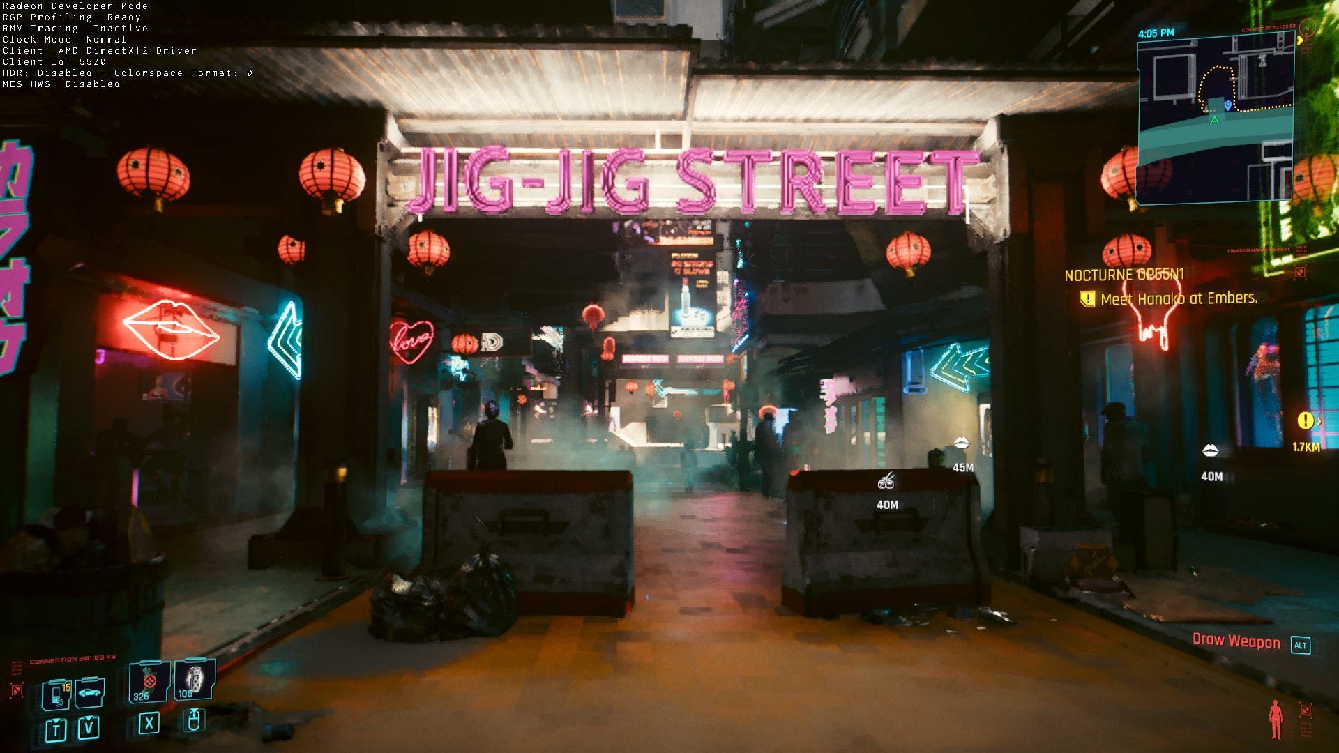
Just like with the previous article, we’re taking a profile while looking down Jig Jig street. With path tracing enabled, the RX 6900 XT struggles along at 5.5 FPS, or 182 ms per frame. Frame time is unsurprisingly dominated by a massive 162 ms raytracing call. Interestingly, there’s still a bit of rasterization and compute shaders at the beginning of the frame. Raytracing calls that correspond to the non-path tracing mode seem to remain as well, but all of that is shoved into insignificance by the gigantic raytracing call added by path tracing mode.
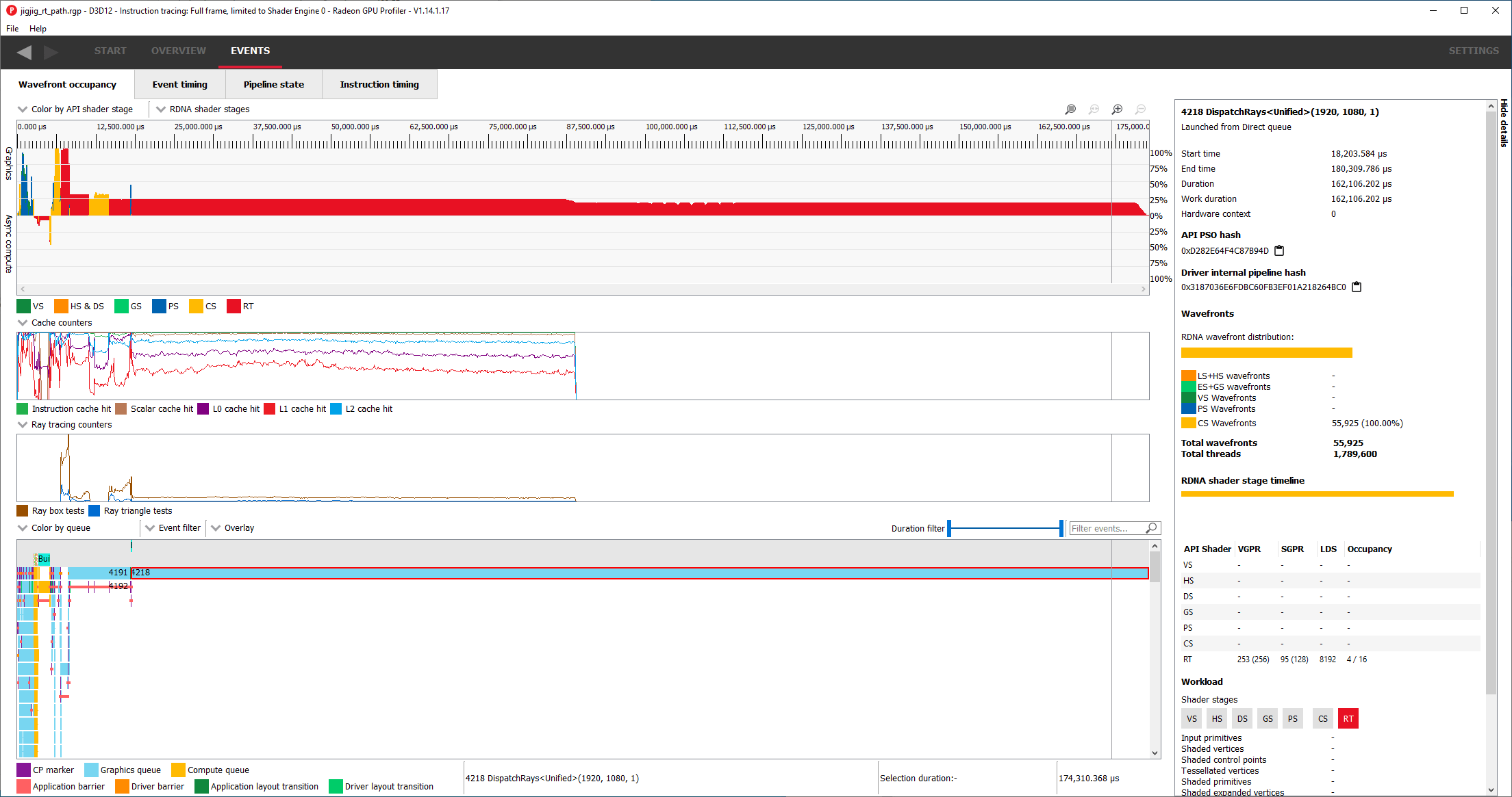
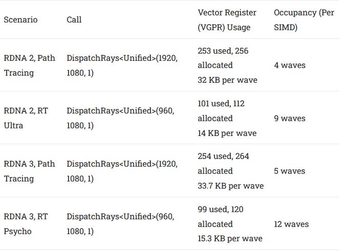
This giant raytracing call generates rays in a 1920×1080 grid, or one invocation per pixel. Looking deeper, the giant raytracing call suffers from poor occupancy. RDNA 2’s SIMDs can track 16 wavefronts, making it a bit like 16-way SMT on a CPU. However, it’s restricted to four wavefronts in this case because each thread uses the maximum allocation of 256 registers per thread. Unlike CPUs, which reserve a fixed number of ISA registers for each SMT thread, GPUs can flexibly allocate registers. But if each thread uses too many registers, it’ll run out of register file capacity and not be able to track as many threads. Technically each thread only asks for 253 registers, but RDNA allocates registers in groups of 16, so it behaves as if 256 registers were used.
Low occupancy means the SIMDs have difficulty finding other work to feed the execution units while waiting on memory accesses. Radeon GPU Profiler demonstrates this by showing how much of instruction latency was “hidden” because the SIMD’s scheduler was able to issue other instructions while waiting for that one to finish.

To be sure, GPU cache latency is absolutely brutal and execution units will almost definitely face stalls even when memory access requests are satisfied from cache. But higher occupancy will usually let a GPU hide more cache latency by finding other work to do while waiting for data to come back.

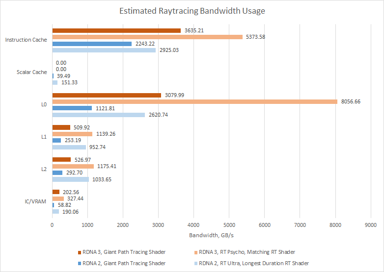
Despite low occupancy, Cyberpunk 2077’s path tracing call achieves decent hardware utilization. A lot of that is thanks to decent cache hitrates. Roughly 96.54% of memory accesses are served from L2 or faster caches, keeping them off the higher latency Infinity Cache and VRAM. Instruction and scalar cache hitrates are excellent. Still, there’s room for improvement. L0 cache hitrate is mediocre at just 65.91%. The L1 has very poor hitrate. It does bring cumulative L0 and L1 hitrate to 79.4%, but there’s a very big jump in latency between L1 and L2.
Long-Tailed Occupancy Behavior
GPUs benefit from a lot of thread-level parallelism, but a task with a lot of threads doesn’t finish until all of the threads finish. Therefore, you want work evenly distributed across your processing cores, so that they finish at about the same time. Usually, GPUs do that reasonably well. However, one shader engine finished its work after 70 ms, leaving a quarter of the GPU idle for the next 91 ms.

I wonder if RT work is a lot less predictable than rasterization workloads, making workload distribution harder. For example, some rays might hit a matte, opaque surface and terminate early. If one shader engine casts a batch of rays that all terminate early, it could end up with a lot less work even if it’s given the same number of rays to start with.
RDNA 3 Improvements, and Raytracing Modes Compared
RDNA 2 has been superseded by AMD’s RDNA 3 architecture, which dramatically improves raytracing performance. I attribute this to several factors. The vector register file and caches received notable capacity increases, attacking the memory access latency problem from two directions (better occupancy and better cache hitrates). New traversal stack management instructions reduce vector ALU load. Dual issue capability further improves raytracing performance by getting through non-raytracing instructions faster. Most of these hardware changes, except for the new traversal stack management instructions, should improve performance for non-raytracing workloads too.

RDNA 3’s SIMDs have a 192 KB vector register file, compared to 128 KB on RDNA 2. That potentially lets RDNA 3 keep more waves in flight, especially if each shader wants to use a lot of registers. Raytracing kernels apparently use a lot of vector registers, so RDNA 3 gains a clear occupancy advantage. Cyberpunk 2077’s path tracing call is especially hungry for vector registers. For comparison, the normal raytracing mode uses far fewer registers and enjoys higher occupancy. It’s also invoked over a grid with half of the screens vertical resolution, probably to make the load lighter.
Alongside a bigger vector register file, RDNA 3 dramatically increases cache sizes. L0 capacity goes from 16 KB to 32 KB, L1 goes from 128 KB to 256 KB, and L2 goes from 4 MB to 6 MB. The result is that 83.2% of requests are handled from L1 or faster caches. Cumulative L2 hitrate doesn’t see a notable improvement. But servicing more requests from within a shader engine means average memory access latency goes down. Combine that with higher occupancy, and RDNA 3 makes better use of bandwidth.
Regular raytracing also enjoys better hardware utilization, across both GPUs. That’s because it gets higher occupancy in the first place, even though its cache hitrates and instruction mix is largely similar. With regular raytracing, hardware utilization on RDNA 2 goes from mediocre to a pretty good level.

Occupancy is a key factor in better hardware utilization, since other characteristics remain similar across the two raytracing workloads. For example, cache hitrates are quite comparable.

RDNA 3 also makes ISA improvements to improve RT core utilization. New LDS (local data share) instructions help raytracing code manage their traversal stack more efficiently. A raytracing acceleration structure is a tree, and traversing a tree involves keeping track of nodes you have to return to, in order to visit their other children.
The local data share is a fast, per-WGP scratchpad memory that offers consistently low latency and high bandwidth, making it an ideal place to store the traversal stack. RDNA 2 uses generic LDS read and write instructions, with a batch of other instructions to manage the stack. RDNA 3 introduces a new LDS instruction that automates traversal stack management.

As a result, RDNA 3 can handle bookkeeping tasks with fewer instructions. Hit count for LDS instructions is nearly halved on RDNA 3 compared to RDNA 2. Looking further at instruction hit counts, RDNA 3 also sees fewer branches compared to RDNA 2. Since the ds_bvh_rtn_stack_b32 instruction takes the address of the last node visited and determines the next node to visit, it possibly avoids branches that we see in RDNA 2 code.

All of these improvements come together to let RDNA 3 make far better use of its intersection test hardware. RDNA 2 was capped at 1.9 GHz here for consistent clocks while RDNA 3 was not. But RDNA 3 is doing intersection tests at a far higher rate than what clock speeds and increased WGP count would account for.

Nvidia’s RTX 4070
Nvidia’s last few generations of video cards have heavily emphasized raytracing. Ada Lovelace, the architecture behind Nvidia’s 4000 series cards, is no exception. Profiling the same Jig Jig street scene reveals that the very long duration path tracing call takes 26.37 ms, which is an excellent performance. For comparison, the RX 7900 XTX took 34.2 ms, though on a different scene. The 6900 XTs is off the charts (in the wrong direction), taking over 160 ms. Part of that is because I ran the card at a locked 1.9 GHz, but increasing clocks by 10-20% would still put RDNA 2’s performance far lower than that of RDNA 3 or Ada.

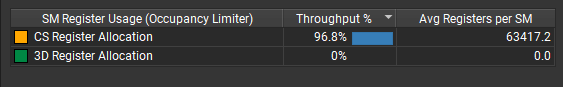
Ada Lovelace’s fundamental building block is the SM, or streaming multiprocessor. It’s roughly analogous to RDNA’s WGP, or workgroup processor. Like a RDNA 2 WGP, an Ada SM has 128 FP32 lanes, split into four partitions. However, each partition only has a 64 KB vector register file, compared to 128 KB on RDNA 2. Maximum occupancy is also lower, at 12 waves per partition compared to 16 on RDNA 2. For the path tracing call, Nvidia’s compiler opted to allocate 124 vector registers, giving the same occupancy as RDNA 2. Each partition only tracks four waves (or warps, in Nvidia’s terminology), basically making a SM or WGP run in SMT-16 mode. I believe Nvidia’s ISA only allows addressing 128 registers, while AMD’s ISA can address 256 registers. So, both Nvidia and AMD’s architectures are nearly maxing out their per-thread register allocations.
Hardware utilization appears similar to that of RDNA 3, though a direct comparison is difficult because of architectural differences and different metrics reported by AMD and Nvidia’s profiling tools. Ada’s SM is nominally capable of issuing four instructions per cycle, or one per cycle for each of its four partitions. The SM averaged 1.7 IPC, achieving 42.7% of its theoretical instruction throughput.

While AMD presents one VALU, or vector ALU, utilization metric, Nvidia has four metrics corresponding to different execution units. According to their profiling guide, FMA Heavy and Light pipelines both handle basic FP32 operations. However, the Heavy pipe can also do integer dot products. The profiling guide also states that the ALU pipe handles integer and bitwise instructions. Load appears to be well distributed across the pipes.
Unfortunately Nsight doesn’t provide instruction-level data like AMD’s Radeon GPU Profiler. However, it does provide commentary on how branches affect performance. RDNA and Ada both use 32-wide waves, which means one instruction applies across 32 lanes. That simplifies hardware, because it only has to track one instruction pointer instead of 32.

It also creates a problem if it hits a conditional branch, and the condition is only true for a subset of those 32 lanes. GPUs handle this “divergence” situation by disabling the lanes for which the condition holds true. In the path tracing call, on average only 11.6 threads were active per 32-wide warp. A lot of throughput is therefore left on the table.

AMD almost certainly faces a similar problem, as it uses similar 32-wide waves. However, Radeon GPU Profiler doesn’t provide stats to confirm this.
On the memory access front, a direct comparison is similiarly infeasible. RDNA has separate paths to its LDS (equivalent to Nvidia’s Shared Memory) and first level data caches. Ada, like many prior Nvidia architectures, can flexibly allocate L1 and Shared Memory capacity out of a single block of SRAM, by varying how much is tagged for use as a cache. LDS or Shared Memory utilization is similiar compared to RDNA 2 (2% for Ada, 3% for RDNA 2), but much lower than the 11.6% for RDNA 3. I suspect RDNA 3’s specialized LDS traversal stack management instructions shove a lot of work to the LDS, and Radeon GPU Profiler reports higher utilization as a result.

From the L1 cache side, utilization is in a good place at 20-30%. Most memory accesses are data access rather than texture ones, which makes sense for a raytracing kernel. L1 hitrate is 67.6%, which surprisingly isn’t as good as I thought it would be. AMD’s RDNA 3 achieves 73.39% L0 hitrate, while RDNA 2 gets 65.9%. Perhaps Ada had to allocate a lot of L1 capacity for use as Shared Memory, meaning it couldn’t use as much for caching.
Once we get to L2, everything looks a lot better for Ada. In a previous article, we noted how Ada’s benefits from excellent caching. Nvidia sticks to two levels of cache, while AMD uses four levels, and therefore enjoys lower latency accesses to Infinity Cache sized memory footprints. The RTX 4070’s L2 cache is substantially smaller than that of flagship products like the 4090, but it still performs very well for Cyberpunk’s path tracing workload. Hitrate is an excellent 97%. L1 already caught 67.6% of memory accesses, so cumulative hitrate to L2 is over 99%.

L2 throughput utilization is 41.9%, which is also a good place to be. Utilization above 70-80% would imply a bandwidth limited scenario, which could definitely be a concern because Ada’s L2 cache has similar capacity to AMD’s Infinity Cache, but has to handle more bandwidth. Thankfully, Nvidia’s L2 cache is very much up to the task. Ada therefore does an excellent job of keeping its execution units fed with a less complex cache hierarchy.
Video Memory Usage
Video memory capacity limitations have a nasty habit of degrading video card performance in modern games, long before their compute power becomes inadequate. Today, it’s especially an issue because there are plenty of very powerful midrange cards equipped with 8 GB of VRAM. For perspective, AMD had 8 GB cards available in late 2015 with the R9 390, and Nvidia did the same in 2016 with the GTX 1080.

With the path tracing “overdrive” mode active, Cyberpunk 2077 allocates 7.1 GB of VRAM. Multi-use buffers are the largest VRAM consumer, eating 4.91 GB. Textures come next, with 2.81 GB. Raytracing-specific memory allocations aren’t too heavy at barely over 400 MB. Path tracing mode does allocate a bit more VRAM than the regular raytracing mode, and most of that is down to multi-use buffers. Those buffers are probably being used to support raytracing, even if Radeon Memory Visualizer doesn’t have enough info to directly attribute them to RT.

While this level of VRAM utilization should be fine for playing the game in isolation, PCs are often used to multitask (unlike consoles). A user could easily have a game walkthrough guide, Discord, and recording software open in the background. They might even be playing a video while gaming. All of those take video memory, and could end up squeezing a 8 GB card.

Thankfully, the situation is less tight with the regular raytracing mode. With 6.66 GB of memory allocated and bound, there should be a decent amount of VRAM left to allow background applications to function properly, or to handle higher resolution texture mods.
Upscaling Technologies
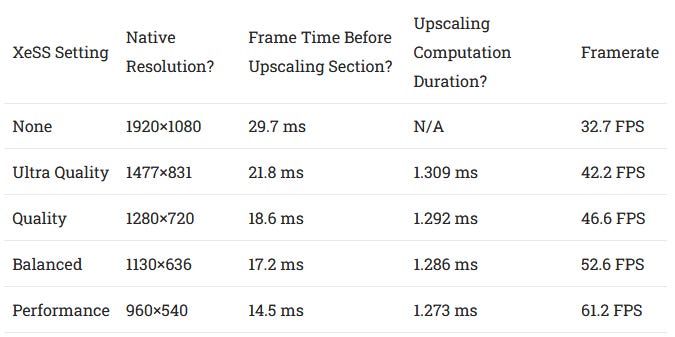
Even limited raytracing effects are still too expensive for the vast majority of video cards in circulation. That’s where upscaling technologies come in. The image is rendered at a lower resolution, and then scaled up to native resolution, hopefully without noticeable artifacts or image quality degradation. Along with path tracing, CD Projekt Red has added support for Intel’s XeSS upscaler. Of course, FSR support remains in place, but the two upscalers can’t be stacked.

Two of the early raytracing calls are dispatched with grid sizes equal to the screen resolution, while the longer duration ones are run with half of the horizontal resolution (giving one invocation per two pixels). Looking those calls gives us a good idea of native rendering resolution.
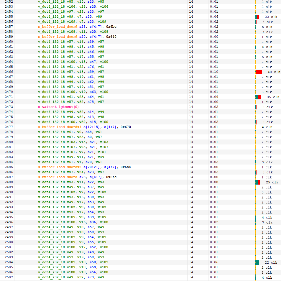
Some of XeSS’s shaders use tons of dot products. Intel says XeSS uses a neural network, we’re probably seeing matrix multiplications used for AI inferencing. v_dot4_i32_i8 instructions treat two 32-bit source registers as vectors of four INT8 elements, computes the dot product, and then adds that with a 32-bit value. AI inferencing often uses lower precision data types, and use of INT8 shows a focus on speed.
However, the longer running XeSS kernels, like one that runs for 0.245 ms, don’t do dot products. Instead, there’s a mix of regular FP32 math instructions, conversions between FP32 and INT32, and texture loads. Machine learning is not as straightforward as applying a batch of matrix multiplications. Data has to be formatted and prepared before it can be fed into a model for inference, and I suspect we’re seeing a bit of that.

XeSS’s calculations take place over about 16 calls, all of which used wave64 mode. Cache hitrates were 70.22%, 7.55%, and 60.84% for L0, L1, and L2 respectively during the XeSS section. Basically, if a request missed L0, it probably wasn’t going to hit L1. Instruction cache hitrate was only 80.86%, indicating that instruction footprints may be large enough to spill out of L1i. Scalar cache hitrate was decent at 95.85%.
Hardware utilization was reasonable even though occupancy was often not a bright spot. If you largely have straight line code full of math instructions, you don’t need a lot of wavefronts in flight to hide memory access latency.

Some of the Dispatch() calls are extremely small. For example, call 5495 only launched 48 wavefronts. The 6900 XT has 160 SIMDs, so a lot of them will be sitting idle with no work to do. Synchronization barriers prevent the GPU from overlapping other work to better fill the shader array, so XeSS has a bit of trouble fully utilizing a GPU as big as the 6900 XT.
After the XeSS section has finished, at least one subsequent DrawInstanced call creates 2,073,601 pixel shader invocations, which corresponds to one thread per pixel for 1920×1080. Even with upscaling in use, some draw calls appear to render at full resolution. These may have to do with UI elements, which take very little time to render regardless of resolution, and have more to lose than gain from upscaling. The same pattern applies to FSR.
Compared to FSR
FSR, or FidelityFX Super resolution, is AMD’s upscaling technology. FSR came out well before XeSS, and was already available in Cyberpunk 2077 before the “Overdrive” patch. Unlike XeSS and Nvidia’s DLSS, FSR does not use machine learning. That also means it doesn’t require specific hardware features like DP4A or matrix multiplication acceleration to perform well. It’s therefore far more widely applicable than Intel or Nvidia’s upsamplers, and can be used on very old hardware.

Compared to XeSS, FSR starts off at lower native resolutions and spends less time doing upscaling computations. That results in higher framerates at similarly labeled quality settings. Like XeSS, FSR uses a set of compute shaders that run in wave64 mode, with synchronization barriers between them. FSR makes even more efficient utilization of compute resources, thanks to higher occupancy and better cache hitrates. In some cases, FSR sees such good hardware utilization that it might be a bit compute bound.

Instruction footprint is lower than with XeSS, bringing instruction cache hitrates back up to very high levels. RDNA 2’s L1 cache does better, but still sees more hits and misses. As with before, the L0 and L2 caches catch the vast majority of accesses. FSR’s memory access patterns are more cache-friendly than XeSS’s in an absolute sense, and that contributes to feeding the execution units.
Unlike XeSS, FSR’s instructions look like a broad mix of vector 32-bit operations with plenty of image memory (texture) instructions mixed in. Math instructions largely deal with FP32 or INT32, unlike XeSS’s use of lower precision with dot products.

I also feel like directly comparing FSR to XeSS is a bit dubious. The two upscalers take different approaches and have different use cases, even though there’s definitely overlap. XeSS employs more expensive upscaling techniques like machine learning, and tends to render at higher native resolutions to start. It’s well suited to modern, high end graphics cards where a moderate framerate bump is enough to go from a slightly low framerate to a playable one. FSR on the other hand starts with lower native resolutions. It uses a brutally fast and efficient upscaling pass that doesn’t rely on specialized operations only available on newer GPUs. That makes it better suited to older or smaller GPUs, where it can deliver a larger framerate increase.
Upscaling on Zen 4’s iGPU
One example of a small GPU is Zen 4’s integrated graphics implementation. Because it’s not meant to handle heavy gaming tasks, it has a single RDNA 2 WGP with 128 FP32 lanes. Caches are tiny as well, with a 64 KB L1 and 256 KB L2. This is the smallest RDNA 2 implementation I’m aware of. I’m testing FSR with raytracing off because performance is already extremely low without raytracing.
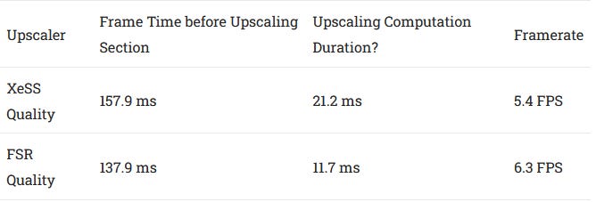
XeSS now takes an extra 10 ms to do its upscaling. Zen 4’s iGPU is extremely compute bound when handling XeSS’s dot product kernels. That highlights a significant weakness of XeSS. Time spent upscaling doesn’t change much regardless of the quality setting, so XeSS provides almost all of its performance boost by allowing the frame to be rendered at lower resolution. On a small GPU, the upscaling time could end up being a significant portion of frame time, putting a low cap on framerate. That makes XeSS less suitable for tiny GPUs, which need upscaling the most.

Another way of looking at it is that XeSS makes excellent use of the iGPU’s compute resources. Earlier, we saw some tiny dispatches that weren’t big enough to fill the 6900 XT’s shader array. With one WGP instead of 40, that’s no longer a problem.
FSR is also extremely compute bound, but has less work to do in the first place. In both cases, we see that filling a small iGPU is a lot easier than doing the same with a large discrete GPU, even though the discrete GPU has a much stronger cache hierarchy.

Even though XeSS and FSR’s “quality” settings appear to use the same native rendering resolution, XeSS spends longer rendering the native frame. One culprit is a very long compute shader toward the middle of the frame. The shader appears to be executing identical code in both cases, but the XeSS frame invoked 28,960 wavefronts (926,720 threads), compared to 28,160 wavefronts (901,120 threads) on the FSR frame. Perhaps there’s more to XeSS and FSR’s differences than just the upscaling pass and native resolution. In any case, we’d need a higher performance preset to run high settings even without raytracing.

Zooming back out, Cyberpunk 2077’s rendering workload is dominated by compute shaders even with raytracing disabled. Vertex and pixel shaders only account for a minority of frame time. Contrast that with indie and older games, where pixel shaders dominate.
Path Tracing on Zen 4’s iGPU?
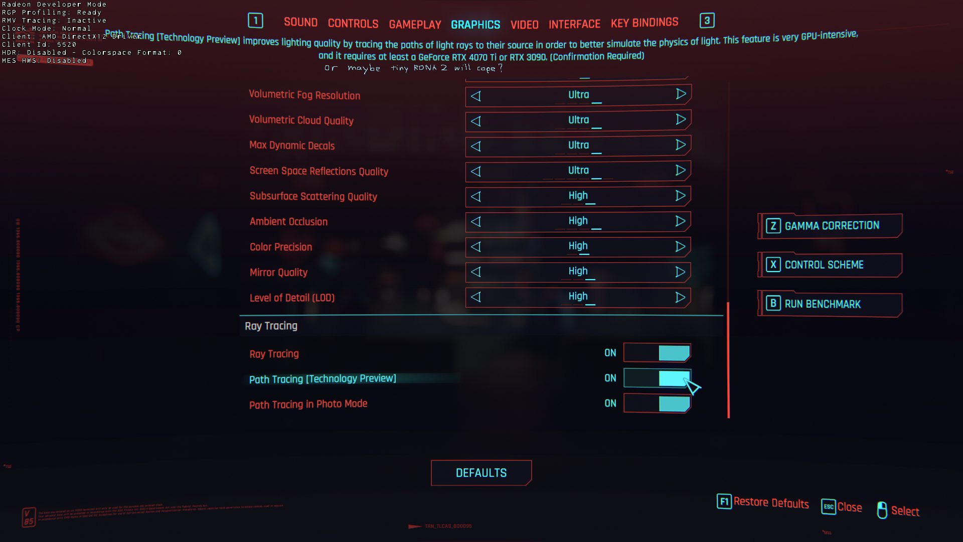
Cyberpunk 2077 explicitly recommends a RTX 4090 or 3090 for the path tracing technology demo. At first glance, this iGPU may not necessarily meet the precise definition put forth by that recommendation. However, after a bit of thinking you may conclude that one WGP is not that much smaller than Van Gogh’s iGPU, which is only a little smaller than the RX 6500XT, which is only a little smaller than the RX 6700XT, which is only a little smaller than the RX 6900 XT, which is only a little smaller than the RX 7900 XTX, which is only a little smaller than the RTX 4090. Because Zen 4’s integrated GPU clearly almost meets the recommended specs, let’s see how it does.
Without FSR, AMD’s profiling tools were unable to take a frame capture at all, even though the GPU was able to render a frame every few seconds. With FSR’s ultra performance mode, Cyberpunk 2077 runs at 4.1 FPS looking down Jig Jig street. The experience is definitely more cinematic than playable. Profiling a frame was difficult too, because the capturing process seems to run out of buffer space and drops events towards the end of the frame. Radeon GPU Profiler’s occupancy timeline only shows 237 out of 243 ms, dropping some data from the end.

Like before, we see a very long duration raytracing call with a bit of long-tailed behavior. However, the long-tailed behavior is nowhere near as bad as it was with the 6900 XT. After all, it’s impossible for one shader engine to finish its work early and sit idle waiting for others to finish, if you only have one shader engine to start with.
Just like on bigger GPUs, frame time is dominated by a huge raytracing call. However, this time it’s a DispatchRays<Indirect> call, not a DispatchRays<Unified> one. The unified DispatchRays call seems to do everything in one large shader without subroutine calls. In contrast, the indirect one uses different functions for ray generation, traversal, and hit/miss handling.

From this, we can see that most of the raytracing cost comes from ray traversal, with ray generation also taking up a significant amount of work. This indirect variation of DispatchRays uses half as many vector registers (128) as the unified path shading kernel from the beginning of the article. That allows each SIMD to track eight waves, instead of just four.
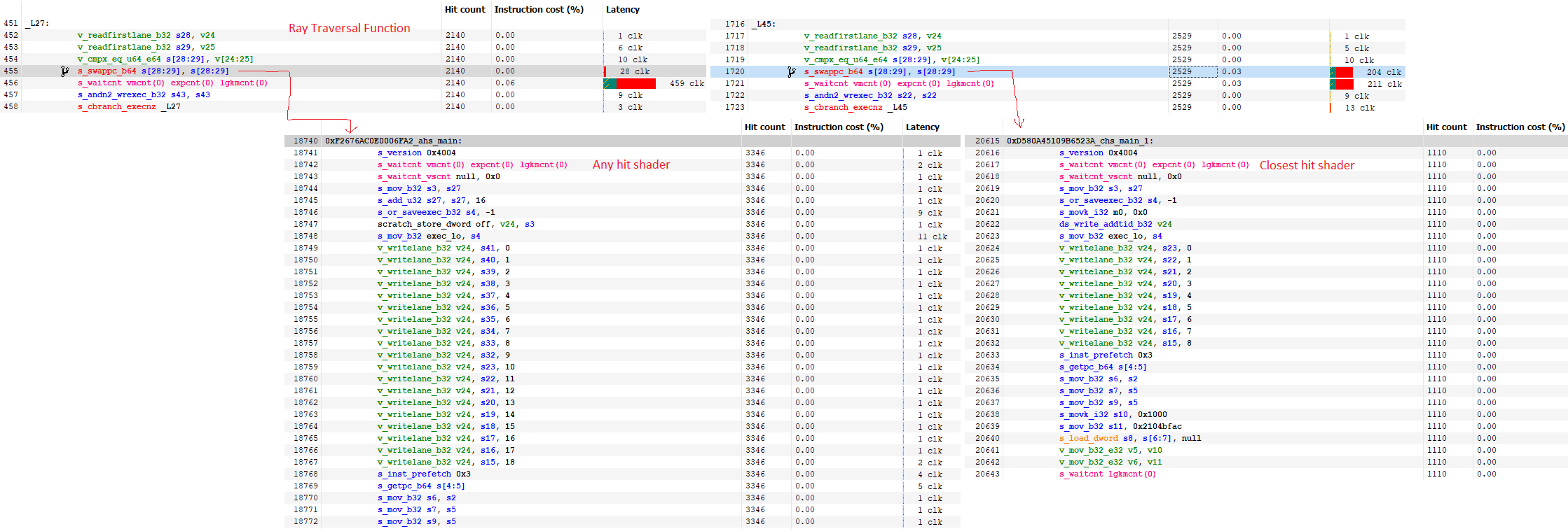
I’m not sure which approach is better. Latency is easier to hide if you have more waves in flight. But function calls incur overhead too. The closest hit/any hit shaders have lengthy prologue and epilogues. s_swappc_b64 and s_setpc_b64 instructions are used to call into and return from functions respectively, and are basically indirect branches. I can’t imagine them being cheap either.

In the end, both approaches achieve similar hardware utilization. The instruction mix is also similar, with roughly one in every hundred executed instructions being a raytracing one. Vector ALU instructions account for about half the executed instructions, while scalar ALU account for just under a quarter of the instruction mix. Just above 10% are branches, so we’re again seeing that raytracing is branchier than other shaders.
FSR’s ultra performance preset is clearly not enough to provide a premium experience on Zen 4’s iGPU.
However, seeing all the lighting effects from Cyberpunk 2077’s technology demo rendered on an iGPU is still amazing, even if pixel-level quality is heavily compromised by upscaling.
Final Words
Raytracing is an expensive but promising rendering technique. Technology demos like Cyberpunk’s show that raytracing has a lot of potential to deliver realistic lighting. However, they also show that we’re still far away from having enough GPU power to make the most of raytracing’s potential. Analyzing Cyberpunk 2077’s Overdrive patch shows that raytracing both requires more work, and harder work. Raytracing sections have more branches and lower occupancy, meaning GPUs face challenges in keeping their execution units fed.
With that in mind, Nvidia’s characterization of raytracing as the “holy grail” of game graphics is a bit inaccurate. The current state of raytracing in games is not the holy grail, as there’s plenty of untapped potential. If you’ve used Blender before, you’ll know that you can increase quality by allowing more ray bounces or getting more samples per pixel (increasing ray count). Furthermore, Cyberpunk 2077’s path tracing mode is so heavy that it has to lean on upscaling technologies to deliver a playable experience.
Cyberpunk’s patch also adds XeSS, which brings our focus to upscaling technologies. FSR and XeSS are the opposite of raytracing. Instead of cutting into performance to deliver more impressive visuals, upscaling seeks to improve framerate with minimal loss to visual quality. Unlike raytracing calls, upscaling requires very little work. On top of that, the upscaling pass runs very efficiently on GPUs. Branches are almost absent. Instead, upscaling uses plenty of straight line code dominated by vector ALU instructions. GPUs love that. Nvidia also has an upscaling technology called DLSS, but we didn’t profile it because Nsight was a pain to get working in the first place for the one trace of Cyberpunk 2077 that we were able to get for this article.
As for upscaling, it’s here to stay for the forseeable future. Real time raytracing is drastically inefficient compared to rasterization. Some of the newest high end cards can use very little upscaling or no upscaling at all, and still deliver raytraced effects at playable framerates. But GPU prices are ridiculous these days. A RTX 4090 sells for over $1600, while the 7900 XTX sells for around $1000. Contrast that with the Pascal generation, where a GTX 1080 sold for $600, and the 1080 Ti went for $700. High end cards are going to be too expensive for a lot of gamers, making upscaling extremely important going forward. Hopefully, advances in both GPU power and upscaling technologies will give us better raytraced effects with very generation.
As a final note, we did try to get data from an A750 as well. However, we couldn’t get a frame capture using Intel’s Graphics Performance Analyzer.
If you like our articles and journalism, and you want to support us in our endeavors, then consider heading over to our Patreon or our PayPal if you want to toss a few bucks our way. If you would like to talk with the Chips and Cheese staff and the people behind the scenes, then consider joining our Discord.